MNIST 上的深度学习

本教程演示如何构建一个简单的前馈神经网络（具有一个隐藏层）并使用 NumPy 从头开始​​训练它以识别手写数字图像。

您的深度学习模型（类似于原始多层感知器的最基本的人工神经网络之一）将学习对MNIST数据集中的 0 到 9 的数字进行分类。该数据集包含 60,000 个训练图像和 10,000 个测试图像以及相应的标签。每个训练和测试图像的大小为 784（或 28x28 像素）——这将是神经网络的输入。

根据图像输入及其标签（监督学习），您的神经网络将被训练以使用前向传播和反向传播（反向模式微分）来学习其特征。网络的最终输出是一个由 10 个分数组成的向量——每个分数对应一个手写数字图像。您还将评估您的模型在对测试集上的图像进行分类方面的表现。

本教程改编自Andrew Trask的作品（已获得作者许可）。

先决条件

读者应该具备一些 Python、NumPy 数组操作和线性代数的知识。此外，您应该熟悉深度学习的主要概念。

要刷新记忆，您可以学习Python和n 维数组上的线性代数教程。

建议您阅读Yann LeCun、Yoshua Bengio 和 Geoffrey Hinton 于 2015 年发表的深度学习论文，他们被认为是该领域的一些先驱。您还应该考虑阅读 Andrew Trask 的Grokking Deep Learning，其中教授如何使用 NumPy 进行深度学习。

除了 NumPy 之外，您还将利用以下 Python 标准模块进行数据加载和处理：

• urllib用于 URL 处理

• request用于打开 URL

• gzip用于gzip文件解压

• pickle使用 pickle 文件格式

  也：

• Matplotlib用于数据可视化

本教程可以在隔离环境中本地运行，例如Virtualenv或conda。您可以使用Jupyter Notebook 或 JupyterLab来运行每个笔记本单元。不要忘记设置 NumPy和Matplotlib。

目录

1. 加载 MNIST 数据集

2. 预处理数据集

3. 从头开始构建和训练小型神经网络

4. 下一步

---

1.加载MNIST数据集

在本部分中，您将下载最初存储在Yann LeCun 网站中的压缩 MNIST 数据集文件。然后，您将使用内置 Python 模块将它们转换为 4 个 NumPy 数组类型的文件。最后，您将把数组分成训练集和测试集。

1.定义一个变量，以列表形式存储 MNIST 数据集的训练/测试图像/标签名称：

data_sources = {
    "training_images": "train-images-idx3-ubyte.gz",  # 60,000 training images.
    "test_images": "t10k-images-idx3-ubyte.gz",  # 10,000 test images.
    "training_labels": "train-labels-idx1-ubyte.gz",  # 60,000 training labels.
    "test_labels": "t10k-labels-idx1-ubyte.gz",  # 10,000 test labels.
}

2.加载数据。首先检查数据是否存储在本地；如果没有，则下载它。

import requests
import os

data_dir = "../_data"
os.makedirs(data_dir, exist_ok=True)

base_url = "https://github.com/rossbar/numpy-tutorial-data-mirror/blob/main/"

for fname in data_sources.values():
    fpath = os.path.join(data_dir, fname)
    if not os.path.exists(fpath):
        print("Downloading file: " + fname)
        resp = requests.get(base_url + fname, stream=True, **request_opts)
        resp.raise_for_status()  # Ensure download was succesful
        with open(fpath, "wb") as fh:
            for chunk in resp.iter_content(chunk_size=128):
                fh.write(chunk)

Downloading file: train-images-idx3-ubyte.gz

Downloading file: t10k-images-idx3-ubyte.gz

Downloading file: train-labels-idx1-ubyte.gz

Downloading file: t10k-labels-idx1-ubyte.gz

3.解压这4个文件并创建 4 ndarrays，并将它们保存到字典中。每个原始图像的大小为 28x28，神经网络通常期望一维向量输入；因此，您还需要通过将 28 乘以 28 (784) 来重塑图像。

import gzip
import numpy as np

mnist_dataset = {}

# Images
for key in ("training_images", "test_images"):
    with gzip.open(os.path.join(data_dir, data_sources[key]), "rb") as mnist_file:
        mnist_dataset[key] = np.frombuffer(
            mnist_file.read(), np.uint8, offset=16
        ).reshape(-1, 28 * 28)
# Labels
for key in ("training_labels", "test_labels"):
    with gzip.open(os.path.join(data_dir, data_sources[key]), "rb") as mnist_file:
        mnist_dataset[key] = np.frombuffer(mnist_file.read(), np.uint8, offset=8)

4.x使用数据和标签的标准表示法将数据拆分为训练集和测试集y，调用训练集和测试集图像x_train和x_test，以及标签y_train和y_test：

x_train, y_train, x_test, y_test = (
    mnist_dataset["training_images"],
    mnist_dataset["training_labels"],
    mnist_dataset["test_images"],
    mnist_dataset["test_labels"],
)

5.您可以确认训练集和测试集的图像数组的形状分别为和，以及标签 -和：(60000, 784)(10000, 784)(60000,)(10000,)

print(
    "The shape of training images: {} and training labels: {}".format(
        x_train.shape, y_train.shape
    )
)
print(
    "The shape of test images: {} and test labels: {}".format(
        x_test.shape, y_test.shape
    )
)

The shape of training images: (60000, 784) and training labels: (60000,)
The shape of test images: (10000, 784) and test labels: (10000,)

6.您可以使用 Matplotlib 检查一些图像：

import matplotlib.pyplot as plt

# Take the 60,000th image (indexed at 59,999) from the training set,
# reshape from (784, ) to (28, 28) to have a valid shape for displaying purposes.
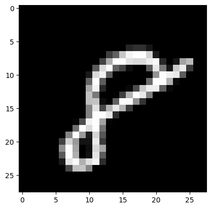
mnist_image = x_train[59999, :].reshape(28, 28)
# Set the color mapping to grayscale to have a black background.
plt.imshow(mnist_image, cmap="gray")
# Display the image.
plt.show()

# Display 5 random images from the training set.
num_examples = 5
seed = 147197952744
rng = np.random.default_rng(seed)

fig, axes = plt.subplots(1, num_examples)
for sample, ax in zip(rng.choice(x_train, size=num_examples, replace=False), axes):
    ax.imshow(sample.reshape(28, 28), cmap="gray")

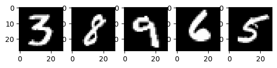
上面是从 MNIST 训练集中获取的五张图像。显示各种手绘阿拉伯数字，每次运行代码时随机选择精确值。

注意：您还可以通过打印将示例图像可视化为数组x_train[59999]。这59999是您的第 60,000 个训练图像样本（0将是您的第一个）。您的输出将相当长，并且应包含一个 8 位整数数组：

...
         0,   0,  38,  48,  48,  22,   0,   0,   0,   0,   0,   0,   0,
         0,   0,   0,   0,   0,   0,   0,   0,   0,   0,   0,   0,   0,
         0,  62,  97, 198, 243, 254, 254, 212,  27,   0,   0,   0,   0,
...

# Display the label of the 60,000th image (indexed at 59,999) from the training set.
y_train[59999]

8

2. 预处理数据

神经网络可以处理浮点类型张量（多维数组）形式的输入。预处理数据时，应考虑以下过程：矢量化和转换为浮点格式。

由于 MNIST 数据已经矢量化并且数组为dtype uint8，您的下一个挑战是将它们转换为浮点格式，例如float64（双精度）：

• 标准化图像数据：一种特征缩放过程，可以通过标准化输入数据的分布来加速神经网络训练过程。

• 图像标签的单热/分类编码。

在实践中，您可以根据您的目标使用不同类型的浮点精度，并且您可以在Nvidia和Google Cloud博客文章中找到更多相关信息。

将图像数据转换为浮点格式

图像数据包含以 [0, 255] 间隔编码的 8 位整数，颜色值在 0 到 255 之间。

您可以将它们除以 255，将它们标准化为 [0, 1] 区间内的浮点数组。

1.检查矢量化图像数据的类型uint8：

print("The data type of training images: {}".format(x_train.dtype))
print("The data type of test images: {}".format(x_test.dtype))

The data type of training images: uint8
The data type of test images: uint8

2.通过除以 255 来标准化数组（从而将数据类型从 提升uint8为float64），然后将训练和测试图像数据变量 —x_train和x_test—分别分配给training_images和train_labels。为了减少本示例中的模型训练和评估时间，将仅使用训练和测试图像的子集。training_images和均test_images仅包含 60,000 张和 10,000 张图像的完整数据集中的 1,000 个样本。这些值可以通过更改 training_sample和 test_sample以下值进行控制，最高可达 60,000 和 10,000 的最大值。

training_sample, test_sample = 1000, 1000
training_images = x_train[0:training_sample] / 255
test_images = x_test[0:test_sample] / 255

3.确认图像数据已更改为浮点格式：

print("The data type of training images: {}".format(training_images.dtype))
print("The data type of test images: {}".format(test_images.dtype))

The data type of training images: float64
The data type of test images: float64

注意：您还可以通过training_images[0]在笔记本单元中打印来检查标准化是否成功。您的长输出应包含浮点数数组：

...
       0.        , 0.        , 0.01176471, 0.07058824, 0.07058824,
       0.07058824, 0.49411765, 0.53333333, 0.68627451, 0.10196078,
       0.65098039, 1.        , 0.96862745, 0.49803922, 0.        ,
...

通过分类/单热编码将标签转换为浮点

您将使用 one-hot 编码将每个数字标签嵌入为全零向量，np.zeros()并放置1标签索引。因此，您的标签数据将是每个图像标签位置带有1.0(或) 的数组。1.

由于总共有 10 个标签（从 0 到 9），因此您的数组将类似于以下内容：

array([0., 0., 0., 0., 0., 1., 0., 0., 0., 0.])

1.确认图像标签数据为整数dtype uint8：

print("The data type of training labels: {}".format(y_train.dtype))
print("The data type of test labels: {}".format(y_test.dtype))

The data type of training labels: uint8
The data type of test labels: uint8

2.定义一个对数组执行one-hot编码的函数：

def one_hot_encoding(labels, dimension=10):
    # Define a one-hot variable for an all-zero vector
    # with 10 dimensions (number labels from 0 to 9).
    one_hot_labels = labels[..., None] == np.arange(dimension)[None]
    # Return one-hot encoded labels.
    return one_hot_labels.astype(np.float64)

3.对标签进行编码并将值分配给新变量：

training_labels = one_hot_encoding(y_train[:training_sample])
test_labels = one_hot_encoding(y_test[:test_sample])

4.检查数据类型是否已更改为浮点：

print("The data type of training labels: {}".format(training_labels.dtype))
print("The data type of test labels: {}".format(test_labels.dtype))

The data type of training labels: float64
The data type of test labels: float64

5.检查一些编码标签：

print(training_labels[0])
print(training_labels[1])
print(training_labels[2])

[0. 0. 0. 0. 0. 1. 0. 0. 0. 0.]
[1. 0. 0. 0. 0. 0. 0. 0. 0. 0.]
[0. 0. 0. 0. 1. 0. 0. 0. 0. 0.]

...并与原件进行比较：

print(y_train[0])
print(y_train[1])
print(y_train[2])

5
0
4

您已完成数据集的准备。

3. 从头开始​​构建并训练一个小型神经网络

在本节中，您将熟悉深度学习模型基本构建块的一些高级概念。您可以参阅原始深度学习研究出版物以获取更多信息。

之后，您将使用 Python 和 NumPy 构建简单深度学习模型的构建块，并训练它学习以一定的准确度识别 MNIST 数据集中的手写数字。

使用 NumPy 构建神经网络模块

• 层：这些构建块充当数据过滤器——它们处理数据并从输入中学习表示，以更好地预测目标输出。

  您将在模型中使用 1 个隐藏层向前传递输入（前向传播）并向后传播损失函数的梯度/误差导数（反向传播）。这些是输入层、隐藏层和输出层。

  在隐藏层（中间层）和输出层（最后层）中，神经网络模型将计算输入的加权和。要计算此过程，您将使用 NumPy 的矩阵乘法函数（“点乘”或）。np.dot(layer, weights)

  注意：为简单起见，本例中省略了偏置项（没有）。np.dot(layer, weights) + bias

• 权重：这些是重要的可调节参数，神经网络通过向前和向后传播数据来进行微调。它们通过称为梯度下降的过程进行优化。在模型训练开始之前，使用 NumPy 随机初始化权重Generator.random()。

  最佳权重应该在训练和测试集上产生最高的预测精度和最低的误差。

• 激活函数：深度学习模型能够确定输入和输出之间的非线性关系，这些非线性函数通常应用于每一层的输出。

  您将使用修正线性单元 (ReLU)来处理隐藏层的输出（例如，.relu(np.dot(layer, weights))

• 正则化：该技术有助于防止神经网络模型过度拟合。

  在此示例中，您将使用一种称为 dropout（稀释）的方法，该方法将图层中的许多特征随机设置为 0。您将使用 NumPy 的Generator.integers()方法定义它并将其应用到网络的隐藏层。

• 损失函数：计算通过将图像标签（真实值）与最终层输出中的预测值进行比较来确定预测的质量。

  为简单起见，您将使用 NumPynp.sum()函数（例如）来使用基本总平方误差。np.sum((final_layer_output - image_labels) ** 2)

• 准确性：该指标衡量网络对其未见过的数据进行预测的能力的准确性。

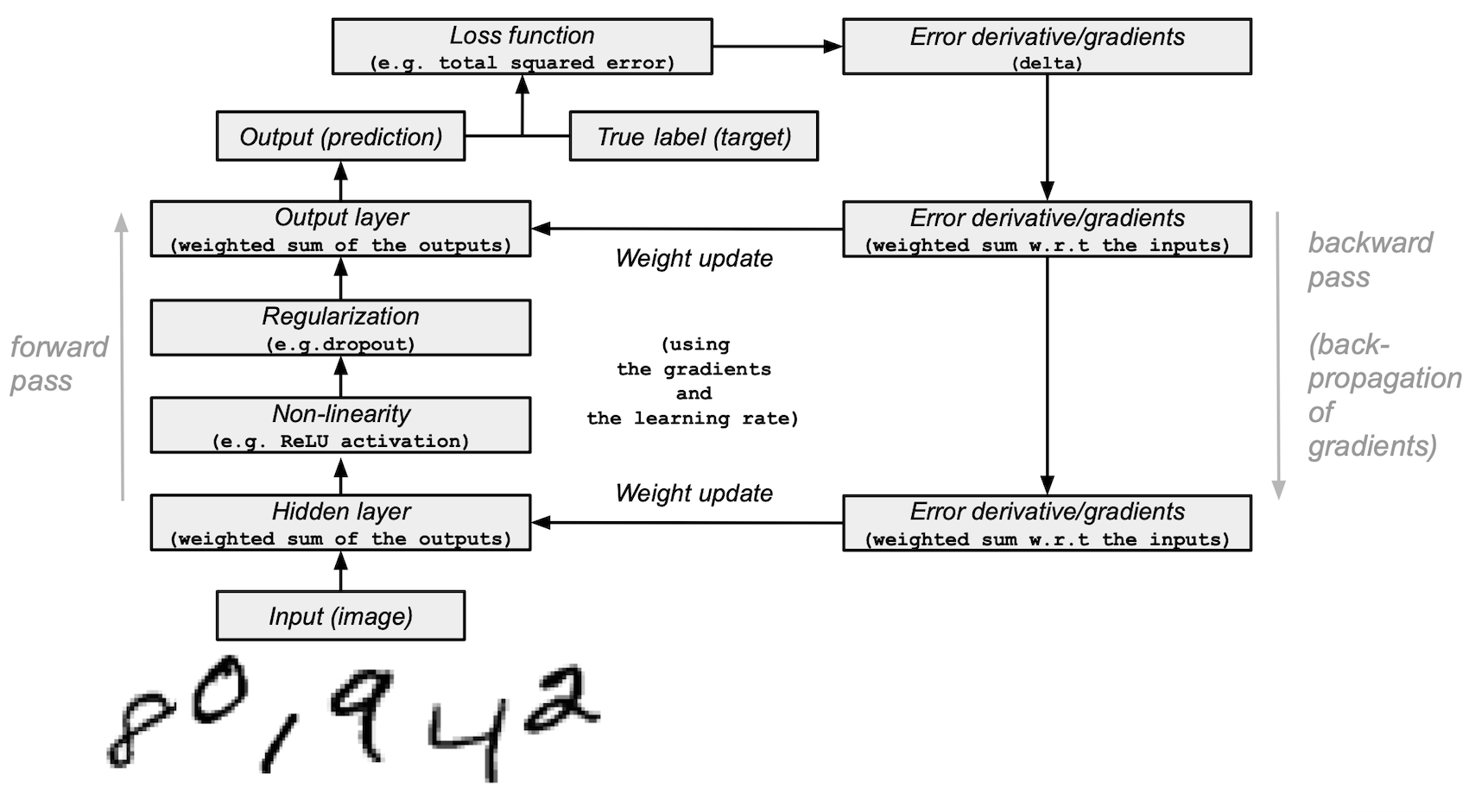
模型架构和训练总结

以下是神经网络模型架构和训练过程的总结：

• 输入层：

  它是网络的输入——之前加载到的预处理training_images数据layer_0。

• 隐藏（中间）层：

  layer_1获取前一层的输出，并通过权重 ( weights_1) 与 NumPy 的np.dot()) 执行输入的矩阵乘法。

  然后，该输出通过 ReLU 激活函数进行非线性处理，然后应用 dropout 来帮助防止过度拟合。

• 输出（最后）层：

  layer_2摄取 的输出layer_1并重复相同的“点乘”过程weights_2。

  最终输出为每个 0-9 数字标签返回 10 个分数。网络模型以大小为 10 的层结束——一个 10 维向量。

• 前向传播、反向传播、训练循环：

  在模型训练开始时，您的网络随机初始化权重并通过隐藏层和输出层向前馈送输入数据。这个过程就是前向传播或前向传播。

  然后，网络将损失函数中的“信号”通过隐藏层传播回来，并借助学习率参数（稍后会详细介绍）调整权重值。

注意：用更专业的术语来说，您：

1. 通过将图像的真实标签（真相）与模型的预测进行比较来测量误差。

2. 对损失函数求微分。

3. 吸收相对于输出的梯度，并相对于通过各层的输入反向传播它们。

由于网络包含张量运算和权重矩阵，因此反向传播使用链式法则。

在神经网络训练的每次迭代（纪元）中，该前向和后向传播循环都会调整权重，这反映在准确性和误差指标中。训练模型时，您的目标是最小化训练数据（模型从中学习）以及测试数据（评估模型）的误差并最大化准确性。

构建模型并开始训练和测试

介绍了主要的深度学习概念和神经网络架构后，让我们编写代码。

1.我们首先创建一个新的随机数生成器，提供可重复性的种子：

seed = 884736743
rng = np.random.default_rng(seed)

2.对于隐藏层，定义用于前向传播的 ReLU 激活函数以及将在反向传播期间使用的 ReLU 导数：

# Define ReLU that returns the input if it's positive and 0 otherwise.
def relu(x):
    return (x >= 0) * x


# Set up a derivative of the ReLU function that returns 1 for a positive input
# and 0 otherwise.
def relu2deriv(output):
    return output >= 0

3.设置某些超参数的默认值，例如：

• 学习率：learning_rate—有助于限制权重更新的幅度，以防止它们过度校正。

• 历元（迭代）：epochs— 数据通过网络的完整传递次数（前向和后向传播）。该参数会对结果产生积极或消极的影响。迭代次数越高，学习过程可能花费的时间就越长。由于这是一项计算密集型任务，因此我们选择了非常少的 epoch 数 (20)。为了获得有意义的结果，您应该选择一个更大的数字。

• 网络中隐藏（中间）层的大小：hidden_size- 隐藏层的不同大小会影响训练和测试期间的结果。

• 输入的大小： pixels_per_image — 您已确定图像输入为 784 (28x28)（以像素为单位）。

• 标签数量：num_labels— 表示输出层的输出数量，其中对 10 个（0 到 9）个手写数字标签进行预测。

learning_rate = 0.005
epochs = 20
hidden_size = 100
pixels_per_image = 784
num_labels = 10

4.使用随机值初始化将在隐藏层和输出层中使用的权重向量：

weights_1 = 0.2 * rng.random((pixels_per_image, hidden_size)) - 0.1
weights_2 = 0.2 * rng.random((hidden_size, num_labels)) - 0.1

5.通过训练循环设置神经网络的学习实验并开始训练过程。请注意，模型会在每个时期根据测试集进行评估，以跟踪其在训练时期的表现。

开始训练过程：

# To store training and test set losses and accurate predictions
# for visualization.
store_training_loss = []
store_training_accurate_pred = []
store_test_loss = []
store_test_accurate_pred = []

# This is a training loop.
# Run the learning experiment for a defined number of epochs (iterations).
for j in range(epochs):

    #################
    # Training step #
    #################

    # Set the initial loss/error and the number of accurate predictions to zero.
    training_loss = 0.0
    training_accurate_predictions = 0

    # For all images in the training set, perform a forward pass
    # and backpropagation and adjust the weights accordingly.
    for i in range(len(training_images)):
        # Forward propagation/forward pass:
        # 1. The input layer:
        #    Initialize the training image data as inputs.
        layer_0 = training_images[i]
        # 2. The hidden layer:
        #    Take in the training image data into the middle layer by
        #    matrix-multiplying it by randomly initialized weights.
        layer_1 = np.dot(layer_0, weights_1)
        # 3. Pass the hidden layer's output through the ReLU activation function.
        layer_1 = relu(layer_1)
        # 4. Define the dropout function for regularization.
        dropout_mask = rng.integers(low=0, high=2, size=layer_1.shape)
        # 5. Apply dropout to the hidden layer's output.
        layer_1 *= dropout_mask * 2
        # 6. The output layer:
        #    Ingest the output of the middle layer into the the final layer
        #    by matrix-multiplying it by randomly initialized weights.
        #    Produce a 10-dimension vector with 10 scores.
        layer_2 = np.dot(layer_1, weights_2)

        # Backpropagation/backward pass:
        # 1. Measure the training error (loss function) between the actual
        #    image labels (the truth) and the prediction by the model.
        training_loss += np.sum((training_labels[i] - layer_2) ** 2)
        # 2. Increment the accurate prediction count.
        training_accurate_predictions += int(
            np.argmax(layer_2) == np.argmax(training_labels[i])
        )
        # 3. Differentiate the loss function/error.
        layer_2_delta = training_labels[i] - layer_2
        # 4. Propagate the gradients of the loss function back through the hidden layer.
        layer_1_delta = np.dot(weights_2, layer_2_delta) * relu2deriv(layer_1)
        # 5. Apply the dropout to the gradients.
        layer_1_delta *= dropout_mask
        # 6. Update the weights for the middle and input layers
        #    by multiplying them by the learning rate and the gradients.
        weights_1 += learning_rate * np.outer(layer_0, layer_1_delta)
        weights_2 += learning_rate * np.outer(layer_1, layer_2_delta)

    # Store training set losses and accurate predictions.
    store_training_loss.append(training_loss)
    store_training_accurate_pred.append(training_accurate_predictions)

    ###################
    # Evaluation step #
    ###################

    # Evaluate model performance on the test set at each epoch.

    # Unlike the training step, the weights are not modified for each image
    # (or batch). Therefore the model can be applied to the test images in a
    # vectorized manner, eliminating the need to loop over each image
    # individually:

    results = relu(test_images @ weights_1) @ weights_2

    # Measure the error between the actual label (truth) and prediction values.
    test_loss = np.sum((test_labels - results) ** 2)

    # Measure prediction accuracy on test set
    test_accurate_predictions = np.sum(
        np.argmax(results, axis=1) == np.argmax(test_labels, axis=1)
    )

    # Store test set losses and accurate predictions.
    store_test_loss.append(test_loss)
    store_test_accurate_pred.append(test_accurate_predictions)

    # Summarize error and accuracy metrics at each epoch
    print(
        (
            f"Epoch: {j}\n"
            f"  Training set error: {training_loss / len(training_images):.3f}\n"
            f"  Training set accuracy: {training_accurate_predictions / len(training_images)}\n"
            f"  Test set error: {test_loss / len(test_images):.3f}\n"
            f"  Test set accuracy: {test_accurate_predictions / len(test_images)}"
        )
    )

Epoch: 0
  Training set error: 0.898
  Training set accuracy: 0.397
  Test set error: 0.680
  Test set accuracy: 0.582

Epoch: 1
  Training set error: 0.656
  Training set accuracy: 0.633
  Test set error: 0.607
  Test set accuracy: 0.641

Epoch: 2
  Training set error: 0.592
  Training set accuracy: 0.68
  Test set error: 0.569
  Test set accuracy: 0.679

Epoch: 3
  Training set error: 0.556
  Training set accuracy: 0.7
  Test set error: 0.541
  Test set accuracy: 0.708

Epoch: 4
  Training set error: 0.534
  Training set accuracy: 0.732
  Test set error: 0.526
  Test set accuracy: 0.729

Epoch: 5
  Training set error: 0.515
  Training set accuracy: 0.715
  Test set error: 0.500
  Test set accuracy: 0.739

Epoch: 6
  Training set error: 0.495
  Training set accuracy: 0.748
  Test set error: 0.487
  Test set accuracy: 0.753

Epoch: 7
  Training set error: 0.483
  Training set accuracy: 0.769
  Test set error: 0.486
  Test set accuracy: 0.747

Epoch: 8
  Training set error: 0.473
  Training set accuracy: 0.776
  Test set error: 0.473
  Test set accuracy: 0.752

Epoch: 9
  Training set error: 0.460
  Training set accuracy: 0.788
  Test set error: 0.462
  Test set accuracy: 0.762

Epoch: 10
  Training set error: 0.465
  Training set accuracy: 0.769
  Test set error: 0.462
  Test set accuracy: 0.767

Epoch: 11
  Training set error: 0.443
  Training set accuracy: 0.801
  Test set error: 0.456
  Test set accuracy: 0.775

Epoch: 12
  Training set error: 0.448
  Training set accuracy: 0.795
  Test set error: 0.455
  Test set accuracy: 0.772

Epoch: 13
  Training set error: 0.438
  Training set accuracy: 0.787
  Test set error: 0.453
  Test set accuracy: 0.778

Epoch: 14
  Training set error: 0.446
  Training set accuracy: 0.791
  Test set error: 0.450
  Test set accuracy: 0.779

Epoch: 15
  Training set error: 0.441
  Training set accuracy: 0.788
  Test set error: 0.452
  Test set accuracy: 0.772

Epoch: 16
  Training set error: 0.437
  Training set accuracy: 0.786
  Test set error: 0.453
  Test set accuracy: 0.772

Epoch: 17
  Training set error: 0.436
  Training set accuracy: 0.794
  Test set error: 0.449
  Test set accuracy: 0.778

Epoch: 18
  Training set error: 0.433
  Training set accuracy: 0.801
  Test set error: 0.450
  Test set accuracy: 0.774

Epoch: 19
  Training set error: 0.429
  Training set accuracy: 0.785
  Test set error: 0.436
  Test set accuracy: 0.784

训练过程可能需要很多分钟，具体取决于许多因素，例如运行实验的机器的处理能力和轮数。为了减少等待时间，您可以将 epoch（迭代）变量从 100 更改为更低的数字，重置运行时间（这将重置权重），然后再次运行笔记本单元。

执行上面的单元格后，您可以可视化此训练过程实例的训练和测试集错误和准确性。

epoch_range = np.arange(epochs) + 1  # Starting from 1

# The training set metrics.
training_metrics = {
    "accuracy": np.asarray(store_training_accurate_pred) / len(training_images),
    "error": np.asarray(store_training_loss) / len(training_images),
}

# The test set metrics.
test_metrics = {
    "accuracy": np.asarray(store_test_accurate_pred) / len(test_images),
    "error": np.asarray(store_test_loss) / len(test_images),
}

# Display the plots.
fig, axes = plt.subplots(nrows=1, ncols=2, figsize=(15, 5))
for ax, metrics, title in zip(
    axes, (training_metrics, test_metrics), ("Training set", "Test set")
):
    # Plot the metrics
    for metric, values in metrics.items():
        ax.plot(epoch_range, values, label=metric.capitalize())
    ax.set_title(title)
    ax.set_xlabel("Epochs")
    ax.legend()
plt.show()

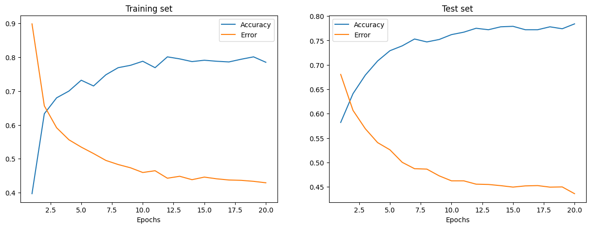
训练和测试误差分别显示在上面的左图和右图中。随着 Epoch 数量的增加，总误差减少，准确度增加。

您的模型在训练和测试期间达到的准确率可能有些合理，但您也可能会发现错误率相当高。

为了减少训练和测试期间的误差，您可以考虑将简单的损失函数更改为例如分类交叉熵。其他可能的解决方案将在下面讨论。

下一步

您已经学习了如何使用 NumPy 从头开始​​构建和训练简单的前馈神经网络来对手写的 MNIST 数字进行分类。

为了进一步增强和优化您的神经网络模型，您可以考虑以下组合之一：

• 将训练样本大小从 1,000 增加到更高的数量（最多 60,000）。

• 使用小批量并降低学习率。

• 通过引入更多隐藏层来改变架构，使网络更深。

• 将交叉熵损失函数与最后一层的softmax激活函数相结合。

• 引入卷积层：用卷积神经网络架构替换前馈网络。

• 使用更大的纪元大小来训练更长的时间，并添加更多的正则化技术，例如提前停止，以防止过度拟合。

• 引入验证集以对模型拟合进行无偏评估。

• 应用批量归一化以实现更快、更稳定的训练。

• 调整其他参数，例如学习率和隐藏层大小。

使用 NumPy 从头开始​​构建神经网络是了解 NumPy 和深度学习更多信息的好方法。然而，对于现实世界的应用程序，您应该使用专门的框架 - 例如PyTorch、JAX、TensorFlow或MXNet - 提供类似 NumPy 的 API，具有内置的自动微分和 GPU 支持，并且专为高性能数值计算和机器学习。

最后，在开发机器学习模型时，您应该考虑潜在的道德问题并应用实践来避免或减轻这些问题：

• 使用模型卡记录经过训练的模型 - 请参阅Margaret Mitchell 等人撰写的用于模型报告的模型卡论文。

• 使用数据表记录数据集 - 请参阅Timnit Gebru 等人的数据集数据表论文）。

• 考虑您的模型的影响 - 谁受其影响，谁受益 - 请参阅Pratyusha Kalluri 的文章和演讲。

• 如需更多资源，请参阅Rachel Thomas 的博客文章和Radical AI 播客。

（感谢hsjeong5演示了如何在不使用外部库的情况下下载 MNIST。）