用 NumPy 中的真实数据确定摩尔定律#

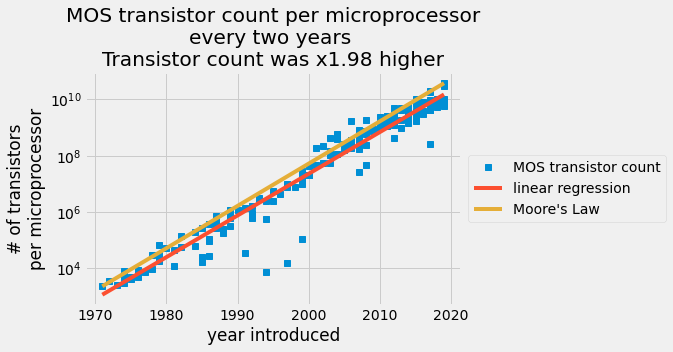
每两年每个微处理器的 MOS 晶体管数量散点图，作为摩尔定律的演示。

每个给定芯片报告的晶体管数量以对数刻度绘制在 y 轴上，引入日期绘制在线性刻度 x 轴上。蓝色数据点来自晶体管计数表。红线是普通的最小二乘预测，橙线是摩尔定律。

你会做什么#

1965 年，工程师戈登·摩尔 (Gordon Moore) 预测，在未来十年中，芯片上的晶体管数量将每两年增加一倍 [ 1 , 2 ]。您将把摩尔的预测与他预测后 53 年内的实际晶体管数量进行比较。您将确定最佳拟合常数来描述半导体晶体管相对于摩尔定律的指数增长。

您将学到的技能#

从*.csv文件加载数据
使用普通最小二乘法执行线性回归并预测指数增长
您将比较模型之间的指数增长常数
在文件中分享您的分析：
- 作为 NumPy 压缩文件*.npz
- 作为*.csv文件
评估半导体制造商在过go五年中取得的惊人进步

你需要什么#

1.这些包：

Numpy
Matplotlib

使用以下命令导入

import matplotlib.pyplot as plt
import numpy as np

2.由于这是指数增长定律，因此您需要一些使用自然对数和指数进行数学计算的背景知识。

您将使用这些 NumPy 和 Matplotlib 函数：

np.loadtxt：此函数将文本加载到 NumPy 数组中
np.log：该函数取 NumPy 数组中所有元素的自然对数
np.exp：该函数采用 NumPy 数组中所有元素的指数
lambda：这是创建函数模型的最小函数定义
plt.semilogy：此函数将 xy 数据绘制到具有线性 x 轴的图形上，并且$\log_{10}$y 轴 plt.plot：此函数将在线性轴上绘制 xy 数据
切片数组：查看加载到工作区中的部分数据，对数组进行切片，例如x[:10]数组中的前 10 个值，x
布尔数组索引：要查看与给定条件匹配的部分数据，请使用布尔运算来索引数组
np.block：将数组组合成二维数组
np.newaxis：将一维向量更改为行向量或列向量
np.savez和np.savetxt：这两个函数将分别以压缩数组格式和文本保存数组

将摩尔定律构建为指数函数#

您的经验模型假设每个半导体的晶体管数量呈指数增长，

$\log(\text{transistor_count})= f(\text{year}) = A\cdot \text{year}+B,$

在哪里$A$和$B$是拟合常数。您可以使用半导体制造商的数据来查找拟合常数。

您可以通过指定添加晶体管的速率 2 并给出给定年份的晶体管初始数量来确定摩尔定律的这些常数。

您以指数形式表述摩尔定律，如下所示，

$\text{transistor_count}= e^{A_M\cdot \text{year} +B_M}.$

在哪里$A_M$和$B_M$是晶体管数量每两年增加一倍的常数，从 1971 年的 2250 个晶体管开始，

$\dfrac{\text{transistor_count}(\text{year} +2)}{\text{transistor_count}(\text{year})} = 2 = \dfrac{e^{B_M}e^{A_M \text{year} + 2A_M}}{e^{B_M}e^{A_M \text{year}}} = e^{2A_M} \rightarrow A_M = \frac{\log(2)}{2}$
$\log(2250) = \frac{\log(2)}{2}\cdot 1971 + B_M \rightarrow B_M = \log(2250)-\frac{\log(2)}{2}\cdot 1971$

所以用指数函数表示的摩尔定律是

$\log(\text{transistor_count})= A_M\cdot \text{year}+B_M,$

在哪里

$A_M=0.3466$

$B_M=-675.4$

由于该函数代表摩尔定律，因此将其定义为 Python 函数： lambda

A_M = np.log(2) / 2
B_M = np.log(2250) - A_M * 1971
Moores_law = lambda year: np.exp(B_M) * np.exp(A_M * year)

1971年，Intel 4004芯片上有2250个晶体管。用于 Moores_law检查戈登·摩尔 (Gordon Moore) 在 1973 年预计的半导体数量。

ML_1971 = Moores_law(1971)
ML_1973 = Moores_law(1973)
print("In 1973, G. Moore expects {:.0f} transistors on Intels chips".format(ML_1973))
print("This is x{:.2f} more transistors than 1971".format(ML_1973 / ML_1971))

In 1973, G. Moore expects 4500 transistors on Intels chips
This is x2.00 more transistors than 1971

将历史制造数据加载到您的工作区#

现在，根据每个芯片的半导体历史数据进行预测。每年的晶体管数量 [4] 都在文件中transistor_data.csv。在将 *.csv 文件加载到 NumPy 数组中之前，最好先检查文件的结构。然后，找到感兴趣的列并将它们保存到变量中。将文件的两列保存到数组data.

在这里，打印出的前 10 行transistor_data.csv。这些列是

处理器	MOS管数量	介绍日期	设计师	MOS工艺	区域
Intel 4004（4位16针）	2250	1971年	英特尔	“10,000纳米”	12平方毫米
……	……	……	……	……	……

! head transistor_data.csv

Processor,MOS transistor count,Date of Introduction,Designer,MOSprocess,Area
Intel 4004 (4-bit  16-pin),2250,1971,Intel,"10,000 nm",12 mm²
Intel 8008 (8-bit  18-pin),3500,1972,Intel,"10,000 nm",14 mm²
NEC μCOM-4 (4-bit  42-pin),2500,1973,NEC,"7,500 nm",?
Intel 4040 (4-bit  16-pin),3000,1974,Intel,"10,000 nm",12 mm²
Motorola 6800 (8-bit  40-pin),4100,1974,Motorola,"6,000 nm",16 mm²
Intel 8080 (8-bit  40-pin),6000,1974,Intel,"6,000 nm",20 mm²
TMS 1000 (4-bit  28-pin),8000,1974,Texas Instruments,"8,000 nm",11 mm²
MOS Technology 6502 (8-bit  40-pin),4528,1975,MOS Technology,"8,000 nm",21 mm²
Intersil IM6100 (12-bit  40-pin; clone of PDP-8),4000,1975,Intersil,,

您不需要指定Processor、Designer、 MOSprocess或Area的列。剩下的第二列和第三列分别是MOS 晶体管数量和引入日期。

接下来，您使用将这两列加载到 NumPy 数组中 np.loadtxt。下面的额外选项会将数据设置为所需的格式：

delimiter = ','：将分隔符指定为逗号“,”（这是默认行为）
usecols = [1,2]：从csv导入第二列和第三列
skiprows = 1：不要使用第一行，因为它是标题行

data = np.loadtxt("transistor_data.csv", delimiter=",", usecols=[1, 2], skiprows=1)

您将半导体的整个历史加载到名为的 NumPy 数组中 data。第一列是MOS 晶体管数量，第二列是四位数年份的推出日期。

year接下来，通过将两列分配给变量和，使数据更易于读取和管理transistor_count。通过使用切片year和transistor_count数组来打印前 10 个值[:10]。打印这些值以检查您是否已将数据保存到正确的变量中。

year = data[:, 1]  # grab the second column and assign
transistor_count = data[:, 0]  # grab the first column and assign

print("year:\t\t", year[:10])
print("trans. cnt:\t", transistor_count[:10])

year:		 [1971. 1972. 1973. 1974. 1974. 1974. 1974. 1975. 1975. 1975.]
trans. cnt:	 [2250. 3500. 2500. 3000. 4100. 6000. 8000. 4528. 4000. 5000.]

您正在创建一个函数来预测给定年份的晶体管数量。您有一个自变量,year和一个因变量, transistor_count。将自变量转换为对数尺度，

$y_i = \log($ transistor_count[i] $),$

得出线性方程，

$y_i = A\cdot \text{year} +B$。

yi = np.log(transistor_count)

计算晶体管的历史增长曲线#

您的模型假设yi是的函数year。现在，找到最小化之间差异的最佳拟合模型$y_i$和$A\cdot \text{year} +B, $像这样

$\min \sum|y_i - (A\cdot \text{year}_i + B)|^2.$

这个误差平方和可以简洁地表示为数组

$\sum|\mathbf{y}-\mathbf{Z} [A,~B]^T|^2,$

在哪里$\mathbf{y}$是一维阵列中晶体管数量的对数的观察值，$\mathbf{Z}=[\text{year}_i^1,~\text{year}_i^0]$是多项式项$\text{year}_i$在第一列和第二列中。通过在中创建这组回归器$\mathbf{Z}-$矩阵你建立了一个普通的最小二乘统计模型。

Z是具有两个参数的线性模型，即次数为的多项式1。因此，我们可以用拟合功能来表示模型numpy.polynomial.Polynomial并使用拟合功能来确定模型参数：

model = np.polynomial.Polynomial.fit(year, yi, deg=1)

默认情况下，Polynomial.fit在由自变量确定的域中执行拟合（year在本例中）。可以使用以下方法恢复未缩放和未平移模型的系数 convert：

model = model.convert()
model

\[x \mapsto \text{-666.32640635} + \text{0.34163208}\,x\]

个别参数$A$和$B$是我们的线性模型的系数：

B, A = model

制造商是否每两年将晶体管数量增加一倍？你有最终的公式，

$\dfrac{\text{transistor_count}(\text{year} +2)}{\text{transistor_count}(\text{year})} = xFactor = \dfrac{e^{B}e^{A( \text{year} + 2)}}{e^{B}e^{A \text{year}}} = e^{2A}$

其中晶体管数量的增加是$xFactor,$年数为 2，并且$A$是半对数函数的最佳拟合斜率。

print(f"Rate of semiconductors added on a chip every 2 years: {np.exp(2 * A):.2f}")

Rate of semiconductors added on a chip every 2 years: 1.98

根据最小二乘回归模型，每个芯片的半导体数量增加了$1.98$每两年一次。您有一个模型可以预测每年的半导体数量。现在将您的模型与实际制造报告进行比较。绘制线性回归结果和所有晶体管计数。

此处，用于 plt.semilogy 以对数刻度绘制晶体管数量，并以线性刻度绘制年份。您已经定义了三个数组来获得最终模型

$y_i = \log(\text{transistor_count}),$

$y_i = A \cdot \text{year} + B,$

和

$\log(\text{transistor_count}) = A\cdot \text{year} + B,$

您的变量 , transistor_count,year和yi都具有相同的维度 , (179,)。 NumPy 数组需要相同的维度才能绘制图。现在预测的晶体管数量是

$\text{transistor_count}_{\text{predicted}} = e^Be^{A\cdot \text{year}}$。

在下图中，使用 fivethirtyeight 样式表。样式表复制 https:// Fivethirtyeight.com 元素。使用更改 matplotlib 样式 plt.style.use。

transistor_count_predicted = np.exp(B) * np.exp(A * year)
transistor_Moores_law = Moores_law(year)
plt.style.use("fivethirtyeight")
plt.semilogy(year, transistor_count, "s", label="MOS transistor count")
plt.semilogy(year, transistor_count_predicted, label="linear regression")


plt.plot(year, transistor_Moores_law, label="Moore's Law")
plt.title(
    "MOS transistor count per microprocessor\n"
    + "every two years \n"
    + "Transistor count was x{:.2f} higher".format(np.exp(A * 2))
)
plt.xlabel("year introduced")
plt.legend(loc="center left", bbox_to_anchor=(1, 0.5))
plt.ylabel("# of transistors\nper microprocessor")

Text(0, 0.5, '# of transistors\nper microprocessor')

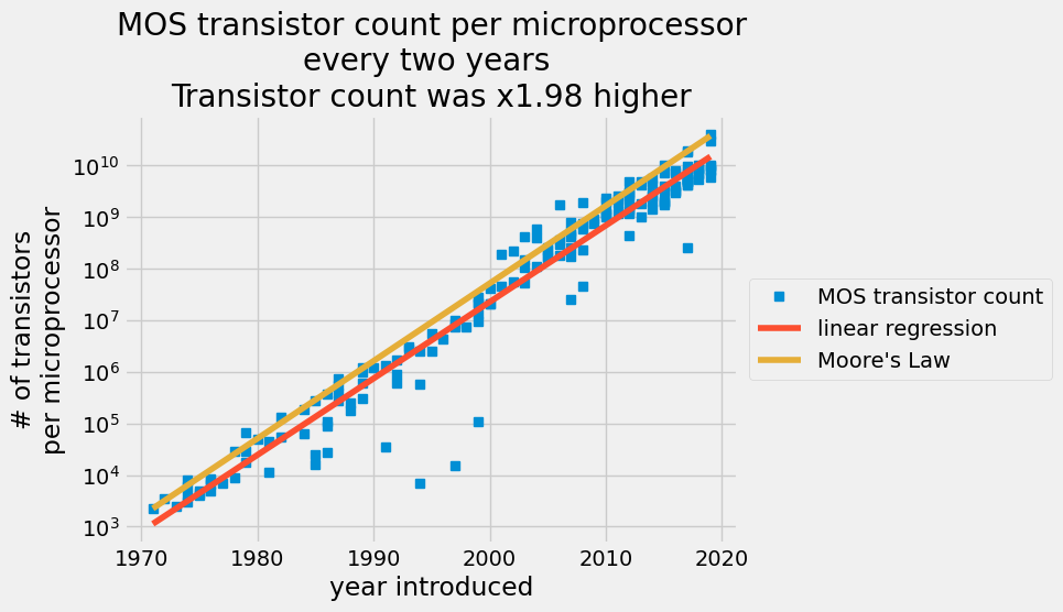
../_images/6b0788a1f2a532ecc631d45fd77e3bd4ac7ed6c3931e2d43430f419028ace14c.png

每两年每个微处理器的 MOS 晶体管数量散点图，其中红线表示普通最小二乘预测，橙色线表示摩尔定律。

线性回归反映了每年每个半导体的晶体管数量的增加。 2015年，半导体制造商声称他们无法再跟上摩尔定律了。您的分析显示，自 1971 年以来，晶体管数量平均每 2 年增加 1.98 倍，但戈登摩尔预测每 2 年将增加 2 倍。这是一个惊人的预测。

考虑 2017 年。将数据与线性回归模型和戈登摩尔的预测进行比较。首先，获取 2017 年的晶体管数量。您可以使用布尔比较器来完成此操作，

year == 2017。

然后，根据上面的定义对 2017 年进行预测Moores_law，并将最适合的常量代入函数中

$\text{transistor_count} = e^{B}e^{A\cdot \text{year}}$。

比较这些测量值的一个好方法是将您的预测和摩尔的预测与平均晶体管数量进行比较，并查看当年报告值的范围。使用 plt.plot 选项 alpha=0.2，可以增加数据的透明度。点越不透明，报告的值就越多。绿色的$+$ 是 2017 年报告的平均晶体管数量。绘制 $\pm\frac{1}{2}~ 年的预测。

transistor_count2017 = transistor_count[year == 2017]
print(
    transistor_count2017.max(), transistor_count2017.min(), transistor_count2017.mean()
)
y = np.linspace(2016.5, 2017.5)
your_model2017 = np.exp(B) * np.exp(A * y)
Moore_Model2017 = Moores_law(y)

plt.plot(
    2017 * np.ones(np.sum(year == 2017)),
    transistor_count2017,
    "ro",
    label="2017",
    alpha=0.2,
)
plt.plot(2017, transistor_count2017.mean(), "g+", markersize=20, mew=6)

plt.plot(y, your_model2017, label="Your prediction")
plt.plot(y, Moore_Model2017, label="Moores law")
plt.ylabel("# of transistors\nper microprocessor")
plt.legend()

19200000000.0 250000000.0 7050000000.0

<matplotlib.legend.Legend at 0x7f864d668460>

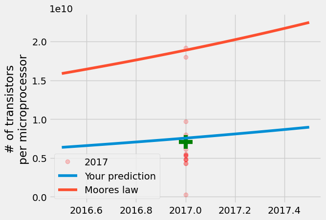
../_images/835ad4be026c38eb31cfff11c655b062e702119cc02d5783e7378d140356433b.png

结果是您的模型接近平均值，但 Gordon Moore 的预测更接近 2017 年生产的每个微处理器的晶体管最大数量。尽管半导体制造商认为增长会放缓，一次是在 1975 年，现在再次临近 2025 年，制造商仍然每两年生产一次半导体，晶体管数量几乎增加一倍。

线性回归模型在预测平均值方面比预测极值要好得多，因为它满足最小化条件$\sum |y_i - A\cdot \text{year}[i]+B|^2$。

包起来＃

总之，您将半导体制造商的历史数据与摩尔定律进行了比较，并创建了一个线性回归模型来查找每两年添加到每个微处理器的晶体管的平均数量。戈登·摩尔 (Gordon Moore) 预测，从 1965 年到 1975 年，晶体管的数量每两年就会翻一番，但平均增长一直保持着稳定的增长$\times 1.98 \pm 0.01$从 1971 年到 2019 年，每两年更新一次。2015 年，摩尔修改了他的预测，称摩尔定律应该持续到 2025 年。[ 3 ]。您可以将这些结果作为压缩的 NumPy 数组文件 mooreslaw_regression.npz或另一个 csv 共享mooreslaw_regression.csv。半导体制造的惊人进步催生了新的产业和计算能力。通过此分析，您应该可以了解过go半个世纪以来这种增长是多么令人难以置信。

用 NumPy 中的真实数据确定摩尔定律

内容

用 NumPy 中的真实数据确定摩尔定律#

你会做什么#

您将学到的技能#

你需要什么#

将摩尔定律构建为指数函数#

将历史制造数据加载到您的工作区#

计算晶体管的历史增长曲线#

包起来＃

参考＃

用 NumPy 中的真实数据确定摩尔定律

内容

用 NumPy 中的真实数据确定摩尔定律#

你会做什么#

您将学到的技能#

你需要什么#

将摩尔定律构建为指数函数#

将历史制造数据加载到您的工作区#

计算晶体管的历史增长曲线#

以压缩数组和 csv 形式共享您的结果#

将数组压缩到文件中#

创建您自己的逗号分隔值文件#

包起来＃

参考＃