numpy.histogram2d

麻木的。histogram2d ( x , y , bins = 10 , range = None , Density = None , Weights = None )

计算两个数据样本的二维直方图。

参数：

x类似数组，形状 (N,)

包含要绘制直方图的点的 x 坐标的数组。

y类似数组，形状 (N,)

包含要绘制直方图的点的 y 坐标的数组。

bins int 或 array_like 或 [int, int] 或 [array, array]，可选

料仓规格：

• 如果是 int，则为二维的 bin 数量 (nx=ny=bins)。

• 如果是 array_like，则为二维的 bin 边缘 (x_edges=y_edges=bins)。

• 如果为 [int, int]，则为每个维度中的 bin 数量 (nx, ny = bins)。

• 如果为 [array, array]，则每个维度中的 bin 边缘 (x_edges, y_edges = bins)。

• 组合 [int, array] 或 [array, int]，其中 int 是 bin 数量，array 是 bin 边缘。

范围array_like，形状（2,2），可选

沿每个维度的 bin 的最左边缘和最右边缘（如果未在bin参数中明确指定）： 。在此范围之外的所有值都将被视为异常值，并且不会在直方图中进行统计。[[xmin, xmax], [ymin, ymax]]

密度bool，可选

如果为 False（默认值），则返回每个 bin 中的样本数。如果为 True，则返回bin 处的 概率密度函数。bin_count / sample_count / bin_area

权重array_like，形状（N，），可选

w_i对每个样本进行称重的一组值。如果密度为 True，则权重标准化为 1 。如果密度为 False，则返回的直方图的值等于属于每个 bin 的样本的权重之和。(x_i, y_i)

返回：

H ndarray，形状（nx，ny）

样本x和y的二维直方图。x中的值 沿第一个维度绘制直方图，y中的值沿第二个维度绘制直方图。

xedges ndarray，形状（nx+1，）

箱沿第一维度边缘。

yedges ndarray，形状（ny+1，）

箱沿第二维边缘。

也可以看看

histogram

一维直方图

histogramdd

多维直方图

笔记

当密度为 True 时，返回的直方图是样本密度，其定义是使产品的 bin 总和 为 1。bin_value * bin_area

请注意，直方图不遵循笛卡尔约定，其中x值位于横坐标，y值位于纵坐标。相反，x沿数组的第一维（垂直）绘制直方图，y沿数组的第二维（水平）绘制直方图。这确保了与 的兼容性histogramdd。

例子

>>> from matplotlib.image import NonUniformImage
>>> import matplotlib.pyplot as plt

构建具有可变 bin 宽度的二维直方图。首先定义 bin 边缘：

>>> xedges = [0, 1, 3, 5]
>>> yedges = [0, 2, 3, 4, 6]

接下来我们创建一个包含随机 bin 内容的直方图 H：

>>> x = np.random.normal(2, 1, 100)
>>> y = np.random.normal(1, 1, 100)
>>> H, xedges, yedges = np.histogram2d(x, y, bins=(xedges, yedges))
>>> # Histogram does not follow Cartesian convention (see Notes),
>>> # therefore transpose H for visualization purposes.
>>> H = H.T

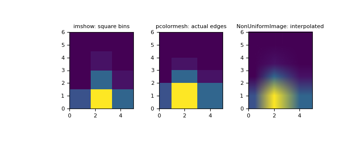
imshow只能显示方形 bin：

>>> fig = plt.figure(figsize=(7, 3))
>>> ax = fig.add_subplot(131, title='imshow: square bins')
>>> plt.imshow(H, interpolation='nearest', origin='lower',
...         extent=[xedges[0], xedges[-1], yedges[0], yedges[-1]])
<matplotlib.image.AxesImage object at 0x...>

pcolormesh可以显示实际边缘：

>>> ax = fig.add_subplot(132, title='pcolormesh: actual edges',
...         aspect='equal')
>>> X, Y = np.meshgrid(xedges, yedges)
>>> ax.pcolormesh(X, Y, H)
<matplotlib.collections.QuadMesh object at 0x...>

NonUniformImage可用于通过插值显示实际的 bin 边缘：

>>> ax = fig.add_subplot(133, title='NonUniformImage: interpolated',
...         aspect='equal', xlim=xedges[[0, -1]], ylim=yedges[[0, -1]])
>>> im = NonUniformImage(ax, interpolation='bilinear')
>>> xcenters = (xedges[:-1] + xedges[1:]) / 2
>>> ycenters = (yedges[:-1] + yedges[1:]) / 2
>>> im.set_data(xcenters, ycenters, H)
>>> ax.add_image(im)
>>> plt.show()

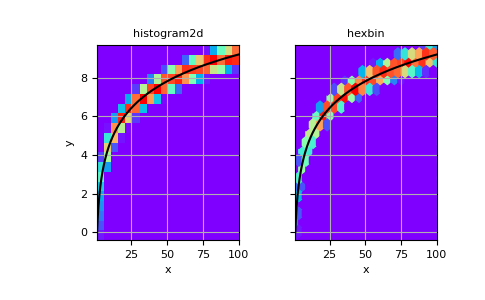
也可以在不指定 bin 边缘的情况下构造二维直方图：

>>> # Generate non-symmetric test data
>>> n = 10000
>>> x = np.linspace(1, 100, n)
>>> y = 2*np.log(x) + np.random.rand(n) - 0.5
>>> # Compute 2d histogram. Note the order of x/y and xedges/yedges
>>> H, yedges, xedges = np.histogram2d(y, x, bins=20)

pcolormesh现在我们可以使用、 和 a 绘制直方图 hexbin以进行比较。

>>> # Plot histogram using pcolormesh
>>> fig, (ax1, ax2) = plt.subplots(ncols=2, sharey=True)
>>> ax1.pcolormesh(xedges, yedges, H, cmap='rainbow')
>>> ax1.plot(x, 2*np.log(x), 'k-')
>>> ax1.set_xlim(x.min(), x.max())
>>> ax1.set_ylim(y.min(), y.max())
>>> ax1.set_xlabel('x')
>>> ax1.set_ylabel('y')
>>> ax1.set_title('histogram2d')
>>> ax1.grid()

>>> # Create hexbin plot for comparison
>>> ax2.hexbin(x, y, gridsize=20, cmap='rainbow')
>>> ax2.plot(x, 2*np.log(x), 'k-')
>>> ax2.set_title('hexbin')
>>> ax2.set_xlim(x.min(), x.max())
>>> ax2.set_xlabel('x')
>>> ax2.grid()

>>> plt.show()